OXYGEN 7.4 – Packed with new tools, instrument improvements and more
The latest OXYGEN 7.4 update brings a wealth of new features, enhancements, and tools designed to improve usability, performance, and analysis capabilities. This version introduces significant upgrades across multiple areas, including OXYGEN-NET, Modal Testing, Power Analysis, Orbit & Polar Plots, and more. Dive into the details below and experience OXYGEN 7.4 for yourself!
New features
Recorder and Chart recorder improvements
OXYGEN-NET improvements
With OXYGEN 7.4 we introduce two major OXYGEN-NET enhancements:
1. Multi-Master mode
OXYGEN-NET supports multiple master clients within a single system. This allows for more complex OXYGEN-NET systems and enables various new features. Key features are:
- Measurement nodes can be configured from different master devices. This means that channel settings, software channels, and further specific settings can be edited from any master device within the same OXYGEN-NET network.
- Introduction of Recording Groups: Every device within an OXYGEN-NET system will be assigned a recording group, which you can edit within the Nodes settings in the tab NET. Different recording groups record data independently from each other even though they use the same measurement nodes.
- Recordings can be controlled from any Master device within the same recording group. Meaning, it is now possible to start a recording on PC1 and pause or stop it on PC2.
Fig. 1 displays an example topology of a Multi-Master system with 3 Slave devices (measurement nodes) and 2 Master devices.
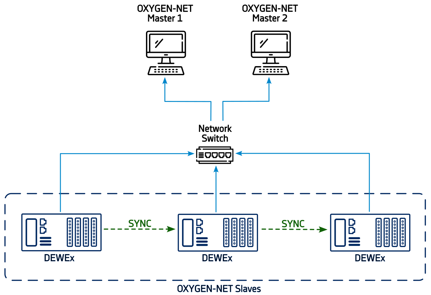
Fig. 1: Example topology of a Multi-Master system
Depending on which recording group the devices are assigned to, there are a wide variety of possible uses. In the following, we describe three cases in more detail:
- Case: Identical recording groups on all devices
- Master 1: Recording Group 1
- Master 2: Recording Group 1
- Slaves: Recording Group 1
In this setup, recordings can be controlled via Master 1 and Master 2. Any recording command (start, pause, and stop measurement) affects all devices, and identical data is stored locally on each device by default.
- Case: Different recording groups on all devices
- Master 1: Recording Group 1
- Master 2: Recording Group 2
- Slaves: Recording Group 3
Here, recording commands only affect the device within the same recording group. For example: A recording started on Master 1 must also be stopped on Master 1, and data is stored only on that device. A recording started on Master 2 functions independently. As only Master devices are able to control recordings, and due to the fact that all Slave devices are within a separate recording group, there will be no data stored on any Slave device.
- Case: Mixed recording groups
- Master 1: Recording Group 1
- Master 2: Recording Group 2
- Slaves: Recording Group 1
In this scenario, a recording command issued on Master 1 will also affect the Slave Unit, resulting in identical data being stored on both devices. Master 2, with a different ID, operates independently.
2. Redundant Master mode
In case a measurement node has multiple LAN ports, a node can now distribute data to multiple master clients simultaneously via multiple networks. Fig. 2 shows an example topology with two independent LAN networks. Both Master devices will receive identical measurement data, however via two different data transfer networks, which enhances the redundancy of the entire system.
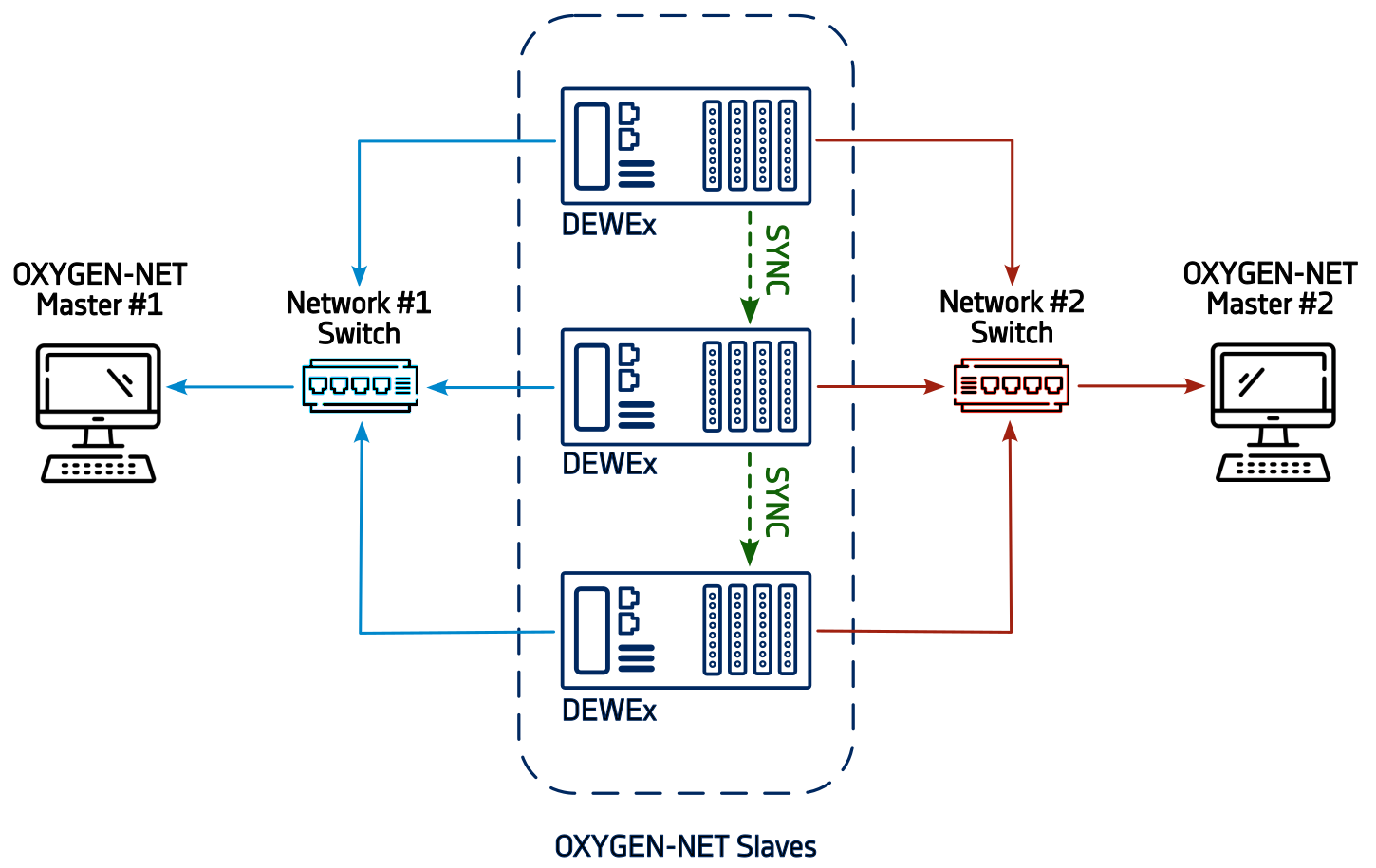
Fig. 2: Redundant Multi-Master system with two LAN networks.
Modal test improvements
One of the key enhancements in our new OXYGEN update is the implementation of the Single Degree Of Freedom(SDOF) Circle Fit method. It is an expansion of our modal test feature and includes new calculation options as well as a new visualization instrument.
Simply put, the SDOF Circle Fit method is a numerical method to estimate the natural frequency and loss factor of a DUT. The method gets its name from its approach: a specific spectral region – where a natural frequency is assumed – is plotted within a Nyquist plot and interpolated into a circle. The resulting intersection of fit and Y-axis shows the exact natural frequency allowing for further calculation of the loss factor.
To visualize a Circle FIT, in we added the Nyquist Instrument ①. This new instrument offers multiple options for selecting the desired frequency range ②, different fitting methods ③, and automatic calculation of the natural frequency and loss factor ④.
The desired frequency range can either be specified manually or linked to instruments. When specified manually, you need to enter a center frequency value. The final frequency range used for visualization is ± 10 bins of this center frequency. In case, you select any “linked to instrument” option, you can further decide to either use a single cursor, two cursors, or three cursors:
- Single cursor method: Allows you to define the center frequency with a single cursor. The system automatically includes 10 bins below and above this center frequency, identical to the manual selection method.
- Dual cursor method: Uses two cursors to define an upper and lower frequency limit. The system then calculates the center frequency as the midpoint of the selected range.
- Triple cursor method: Enables an asymmetrical selection by using three cursors to define the lower, center, and upper-frequency values
Regarding fitting methods, three options are available:
- Off: no fitting will be performed and therefore no calculation of the natural frequency nor loss factor
- Center only: A fitting routine in which the fitted radius always passes through the origin of the coordinate system [0|0]. The natural frequency and loss factor are calculated automatically.
- Center and radius: A different fitting routine in which the fitted radius does not need to cross the origin of the coordinate system [0|0]. The natural frequency and loss factor are calculated automatically.
Additionally, we have added a new screen template for Modal Test that includes the Circle Fit visualization, named “ModalTest: Nyquist“.
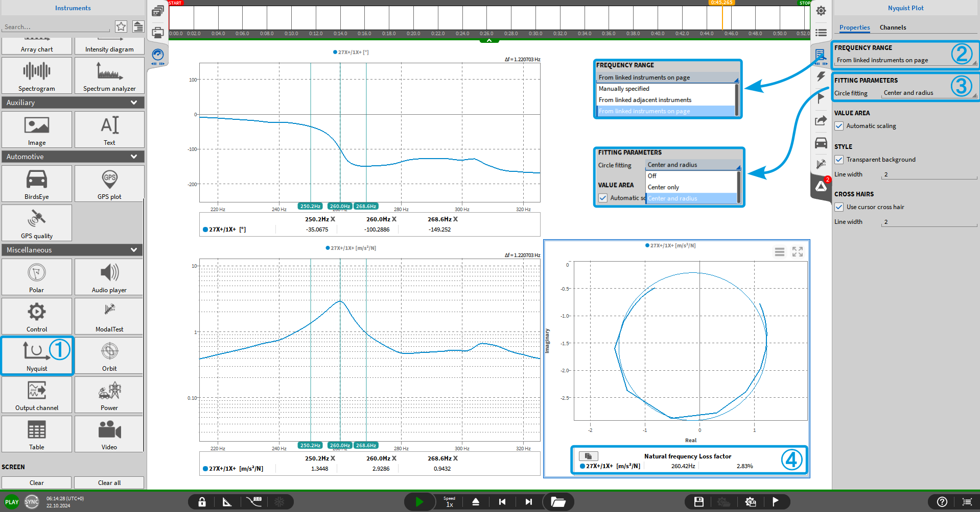
Fig. 3: Measurement screen highlighting the Nyquist Instrument
Beyond the Circle Fit feature, we further added the possibility to export the modal shape animation as video (*.mkv). Therefore, we added a VIDEO EXPORT section to the Modal Test instrument properties. In this section, you can define the number of animation cycles and decide if they want to export only the instrument or the entire measurement screen. Note that the export of the modal shape animation is available in PLAY mode, not in LIVE mode.
Note: The Modal Test feature, including all its functionalities, requires the OXY-OPT-MODAL option.
Orbit plot & Polar plot
OXYGEN 7.4 introduces two powerful new instruments for orbit analysis: the Orbit instrument and the Polar instrument. These tools are especially useful for diagnosing rotational machinery issues by visualizing shaft movement and vibration patterns.
Orbit Instrument
The Orbit Instrument generates an orbit plot, which illustrates the movement of a shaft in rotating machinery. In an ideal system, the shaft centerline remains stationary; however, real-world factors cause vibrations that can be visualized using this tool. The Orbit Instrument provides several display options that can be combined for a comprehensive analysis:
- Raw orbit & Average orbit: Displays the real-time movement of the shaft center. Grey lines represent individual orbits, while the bold black line shows the average orbit. Required inputs: X and Y movements. For meaningful interpretation, an angle and speed (RPM) signal are recommended.
- Centerline plot: Captures snapshots of the movement center at user-defined RPM intervals. Required inputs: X movement, Y movement, angle, and speed signals.
- Filtered orbit: Displays a filtered movement in form of extracted orders of the live shaft movement. Required inputs: X movement, Y movement, angle, and speed signals. Additionally, for each order, amplitude and phase data for the X and Y signals must be assigned. Note: The OXY-OPT-OA (Order Analysis) option is required for extracting order information.
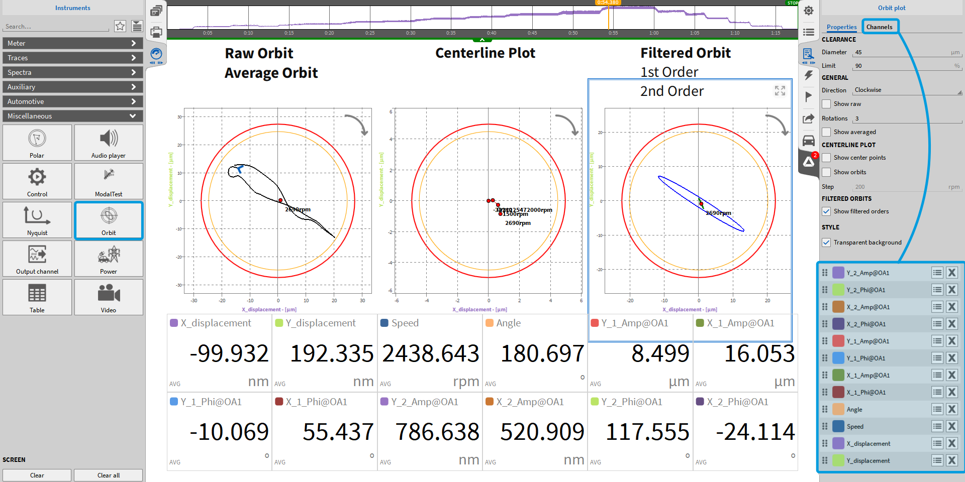
Fig. 4: Example measurement screen with three orbit plots
Fig. 4 illustrates an example measurement screen featuring three distinct orbit plots. In the instrument tab (left column), the Orbit Instrument is highlighted. On the right side, the instrument properties are displayed, along with the assigned channels for the plot labeled Filtered Orbit. For detailed settings, configurations, and examples, refer to the OXYGEN manual or online help.
Polar instrument
The Polar instrument generates a polar plot, which is used to display vector signals in polar coordinates. This is particularly useful for visualizing the amplitude and phase relationships of signals. For example, it can display the amplitude and phase of a user-defined order of X-deflection at a given shaft speed. In general, in the polar plot, the amplitude is represented as the radius, indicating the magnitude of the signal, whereas the phase is represented as the angle, showing the signal’s phase shift. The polar instrument requires three input channels: a speed signal, and the amplitude and phase information of the desired signal. In OXYGEN, for instance, amplitude and phase data for specific signal orders can be extracted via the order analysis feature.
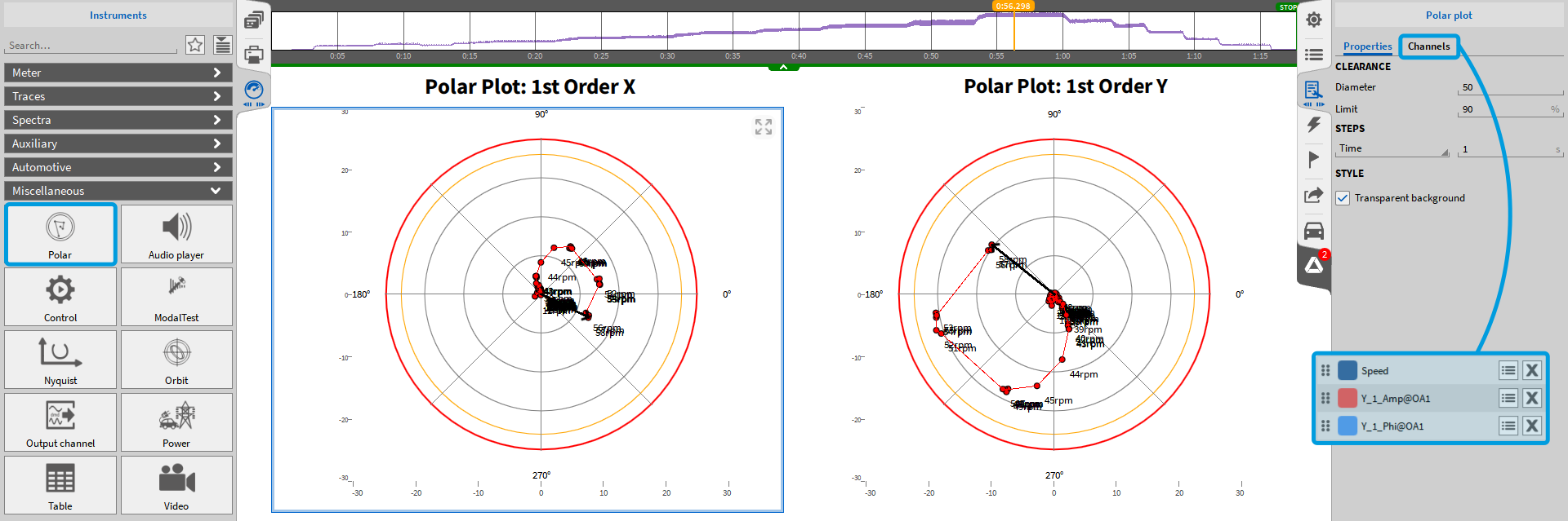
Fig. 5: Example measurement screen with two polar plots showing the amplitude and phase of the first order
Fig. 5 illustrates an example measurement screen showing two polar plots – once for the extracted 1st order of the X deflection, and once for the extracted 1st order of the Y deflection. In the instrument tab (left column), the Polar Instrument is highlighted. On the right side, the instrument properties are displayed, along with the assigned channels for the plot labeled Polar Plot: 1st Order X. For detailed settings, configurations, and examples, refer to the OXYGEN manual or online help.
Recorder and Chart recorder improvements
New marker functionality
You can now add up to ten markers in the Recorder or Chart Recorder, either by clicking directly in the Recorder or via a dedicated button ① in the instrument properties. These markers simply display the channel value at the marker position. The resulting marker table ② can be copied to the clipboard for easy sharing and documentation. Further, these markers can be renamed and shifted across the entire time axis. This feature is available in LIVE (Freeze), REC (DéjàView), and PLAY modes.
Customizable cursor table layout
The cursor table ③ can now be split into 1, 2, 3, or 4 columns, allowing you to adjust the layout according to their needs. To do so check the Cursor section within the instrument properties and select the desired amount of visible columns ④.
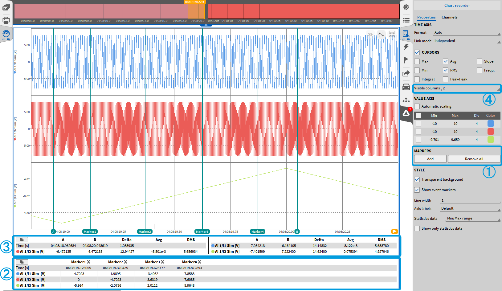
Fig. 6: Chart recorder instrument with marker table ② and cursor table ③
Text instrument improvements
With OXYGEN 7.4 we further introduced new Text Instrument improvements to enhance usability, customization, and data presentation. The new update enables you to apply advanced text formatting to specific words or characters instead of formatting the entire textbox. This feature must be enabled via the checkbox “Allow advanced formatting” ① in the instrument properties. The available formatting options ② include:
- Line break
- Italic style for individual characters or words
- Bold style for individual characters or words
- Preformatted text to ensure identical line indentation
- subscript for individual characters or words
- superscript for individual characters or words
Additionally, the Text Instrument now supports the visualization of measurement start and end times ③. You can simply drag and drop this information from the instrument’s properties menu.
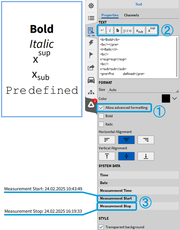
Fig. 7: Text Instrument enhancements
Power improvements
OXYGEN now offers the flexibility to calculate relative harmonics using either the fundamental value as a reference or the nominal value as a reference. Previously, the fundamental value was used as the reference, whereas now you can alternatively select the nominal value as the reference. This selection applies to voltage harmonics, current harmonics, as well as interharmonics.
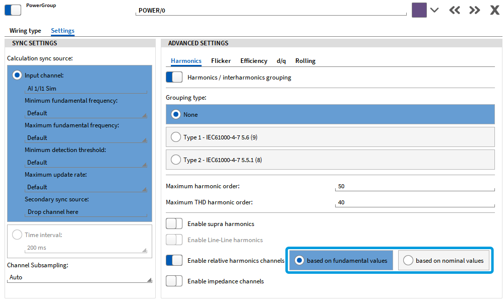
Fig. 8: New calculation option for relative harmonics for power analysis
New SCPI commands
New OXYGEN, new SCPI commands – with this update, we provide multiple new SCPI commands to query detailed information about Sync In/Out settings:
- :SYNC:STATe? Query the current synchronization hardware state (exists since R5.5)
- :SYNC:ENCLOSURES:LIST? Returns the most important information about all enclosures in the system.
- :SYNC:ENClosure#:NAMe? Returns the name of the selected enclosure
- :SYNC:ENC#:SERial? Returns the serial number of the selected enclosure
- :SYNC:ENC#:NODEName? Returns the name of the parent node of the selected enclosure
- :SYNC:ENC#:IN:MODe? Returns the current mode of the synchronization input
- :SYNC:ENC#:OUTPUTS:LIST? Returns information about the sync output connectors of the selected enclosure
- :SYNC:ENC#:OUT#:NAMe? Returns the name of the specified synchronization output
- :SYNC:ENC#:OUT#:CONnector? Returns the connector name of the specified synchronization output
- :SYNC:ENC#:OUT#:MODe? Returns the current mode of the specified synchronization output connector
For details refer to our SCPI command reference document or SCPI online help.
Reporting updates
Our reporting tool now supports two additional paper sizes—DIN A5 (148 x 210 mm) and A6 (105 x 148 mm), which can be selected within the Page Settings in the Reporting section. Additionally, we have removed the DEWETRON footer icon from the default report page for a cleaner and more customizable layout.
Additional improvements
Saturation meter instrument
We introduce a reset option for all channels within the Saturation Meter instrument, allowing you to clear values with a single button click. This can be done either via the on-measurement screen instrument settings ① or through the control instrument ②.
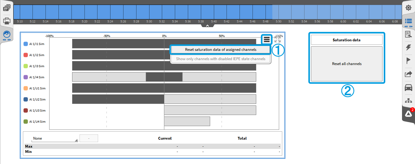
Fig. 9: Reset all saturation meter channels
Synchronization of XR-data
Synchronization of acquired XR data is now possible when using via CAN connection. This includes synchronization between multiple XR modules as well as synchronization with other system signals such as analog signals, math channels, etc. To enable synchronous data acquisition, you must select the “Synchronous output channels” checkbox when adding XR modules to the OXYGEN channel list. This ensures that the acquired XR data has equidistant timestamps, perfectly aligned with the system data.
Usability and operability improvements
Our latest update enhances the user-friendliness and workflow efficiency in OXYGEN with several minor improvements:
- Drag-and-Drop System Assignment: you can now assign entire systems or boards to instruments on the measurement screen via drag-and-drop, rather than assigning individual channels one by one.
- Toggle Design Mode Via Mouse Button: Quickly toggle the Design Mode using the middle mouse button.
- Enhanced Simplified XML Setup: You can define screen templates within a *simplified .xml setup.
- DMD-File Enhancements: .dmd files now include information about the .dms file used for the measurement. This information is readily available when opening a .dmd file, ensuring better traceability and data management.
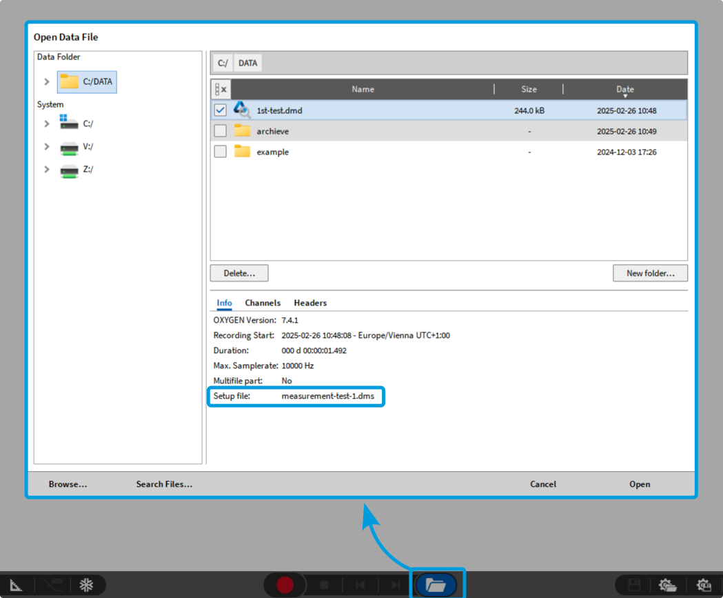
Fig. 10: Setup file information when loading .dmd files
Channel setting enhancements
OXYGEN 7.4 introduces new configuration options and settings for both hardware and software channels:
- Bridge Balancing for TRION(3)-18xx-MULTI: You can now enter the shunt target value in engineering units when sensor scaling is active.
- Two Pulse Edge Separation Mode for Counter channels: Allows measurement of the time between a rising edge on Input A and Input B. Note that two counter input channels are required. For more details, refer to the TRION Technical Reference Manual.
- Math FFT – Optimized Complex FFT Handling: You can now reduce complex FFT channels to specific frequency bins. Only the defined frequency bins are extracted, while all other data are discarded. This applies to all FFT output channels, including phase channels. The key benefit of bin reduction is a significant decrease in RAM and CPU usage, making it especially useful when handling a large number of FFTs.
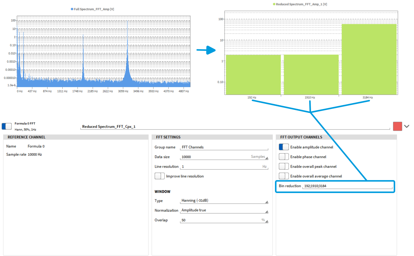
Fig. 11: Bin reduction for Math FFT